Vertical Lift Performance
Definition: The Vertical Lift Performance (VLP) describes the relationship between the bottom-hole flowing pressure (\(p_{wf}\)) and the production rate (\(q\)). It represents the pressure required to lift fluids from the bottom-hole to the surface against gravity, friction, and acceleration.
Oil Well VLP (Single Phase)
For a single-phase liquid, the pressure gradient (\(dp/dz\)) is the sum of hydrostatic (elevation) and frictional components.
Differential Equation:
Where: - \(\rho\) = fluid density (\(lb/ft^3\)) - \(g\) = gravitational constant - \(f\) = Fanning friction factor - \(v\) = fluid velocity (\(ft/s\)) - \(D\) = tubing internal diameter (\(ft\))
Numerical Example (ODEs with SepalSolver): We solve for \(p_{wf}\) by integrating from surface pressure (\(p_{surf}\)) to the total depth (\(H\)).
// Inputs
double p_surf = 200; // psi (Wellhead Pressure)
double depth = 2000; // ft
double q_o = 500; // STB/day
// ODE Definition: dp/dz = gradient
double pressureGradient(double z, double p, double q)
{
double density = 55.0; // lb/ft3 (Oil)
double friction_grad = 0.00002 * Pow(q, 1.8); // Simplified friction term
double hydro_grad = density / 144.0; // psi/ft
return hydro_grad + friction_grad;
}
// Solve using SepalSolver Ode45
// Integrate from z=0 (surface) to z=8000 (bottom-hole)
var (Z, P) = Ode45((z, p)=>pressureGradient(z, p, q_o), p_surf, [0, depth]);
double p_wf = P[^1]; // extract the pressure at the bottom
Console.WriteLine($"Bottom-hole Flowing Pressure (Pwf) = {p_wf:F2} psi");
//FullRange
double pfun(double q_g)
{
var (Z, P) = Ode45((z, p) => pressureGradient(z, p, q_g), p_surf, [0, depth]);
double p_wf = P[^1]; // extract the pressure at the bottom
return p_wf;
}
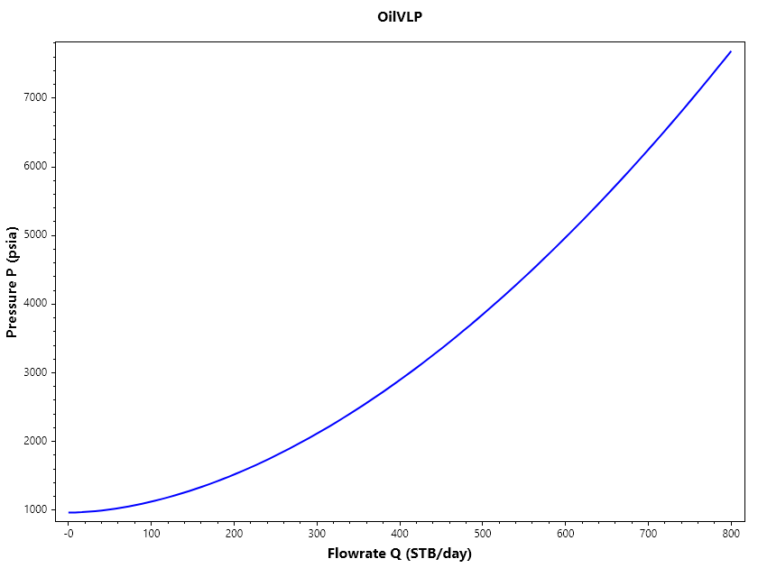
ColVec Qrange = Linspace(0, 800);
ColVec Prange = Arrayfun(pfun, Qrange);
Plot(Qrange, Prange, "b", 2);
Xlabel("Flowrate Q (STB/day)");
Ylabel("Pressure P (psia)");
Title("OilVLP");
SaveAs("OilVLP.png");
Ouput
Bottom-hole Flowing Pressure (Pwf) = 3849.29 psi
Gas Well VLP
Gas VLP is more complex because gas density is highly dependent on pressure. As gas rises, it expands, increasing velocity and frictional losses.
Differential Equation:
Numerical Example (ODEs with SepalSolver): In this example, the gradient function must recalculate gas density (\(\rho_g = \frac{p M}{Z R T}\)) at every step of the integration.
double p_surf = 500; // psia
double depth = 10000; // ft
double q_g = 5000; // Mscf/day
// ODE Definition for Gas
double pressureGradient(double z, double p, double q)
{
double MW = 20.0; // Gas molecular weight
double T = 540 + (0.015 * z); // Temp profile in Rankine
double Z = 0.85; // Average Z-factor
double R = 10.73;
// Density as a function of current Pressure (p)
double rho_g = (p * MW) / (Z * R * T);
double hydro_grad = rho_g / 144.0;
double friction_grad = 1.5e-9 * (Pow(q, 2) / p); // Simplified gas friction
return hydro_grad + friction_grad;
}
// Solve using SepalSolver Ode45
// Integrate from z=0 (surface) to z=8000 (bottom-hole)
var (Z, P) = Ode45((z, p)=>pressureGradient(z, p, q_g), p_surf, [0, depth]);
double p_wf = P[^1]; // extract the pressure at the bottom
Console.WriteLine($"Bottom-hole Flowing Pressure (Pwf) = {p_wf:F2} psi");
//FullRange
double pfun(double q_g)
{
var (Z, P) = Ode45((z, p) => pressureGradient(z, p, q_g), p_surf, [0, depth]);
double p_wf = P[^1]; // extract the pressure at the bottom
return p_wf;
}
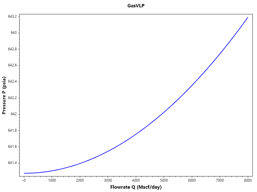
ColVec Qrange = Linspace(0, 8000);
ColVec Prange = Arrayfun(pfun, Qrange);
Plot(Qrange, Prange, "b", 2);
Xlabel("Flowrate Q (Mscf/day)");
Ylabel("Pressure P (psia)");
Title("GasVLP");
SaveAs("GasVLP.png");
Ouput
Bottom-hole Flowing Pressure (Pwf) = 642.03 psi