Gas Reservoir Material Balance
Definition: The Gas Material Balance equation (GMBE) is based on the principle of conservation of mass. For a volumetric gas reservoir (no water drive), the relationship between reservoir pressure and cumulative production is linear when expressed as \(p/z\) vs. \(G_p\).
The p/z Equation
For a volumetric reservoir, the relationship is defined as:
Where:
\(p\) = current average reservoir pressure (psia)
\(z\) = gas deviation factor at pressure \(p\)
\(p_i, z_i\) = initial reservoir pressure and gas deviation factor
\(G_p\) = cumulative gas production (Bscf)
\(G\) = Original Gas-In-Place (OGIP) (Bscf)
Numerical Example:
Given:
\(p_i = 4000 \, \text{psia}, z_i = 0.91\)
\(G = 100 \, \text{Bscf}\)
Current \(G_p = 20 \, \text{Bscf}\)
Current \(z = 0.88\)
double G = 100; // Bscf (OGIP)
double Gp = 20; // Bscf (Produced)
double pi = 4000; // psia
double zi = 0.91;
double z_current = 0.88;
double p_over_z = (pi / zi) * (1 - (Gp / G));
double p_current = p_over_z * z_current;
Console.WriteLine($"Current Reservoir Pressure (p) = {p_current:F2} psia");
Ouput
Current Reservoir Pressure (p) = 3094.51 psia
Material Balance with Water Drive
If an active aquifer is present, water influx (\(W_e\)) maintains reservoir pressure, causing the \(p/z\) plot to deviate from a straight line.
General Equation:
Numerical Example (Solving for OGIP with Water Influx):
double Gp = 15.0; // Bscf
double Bg = 0.00085; // res ft3/scf (Current)
double Bgi = 0.00072; // res ft3/scf (Initial)
double We = 2.5e6; // res ft3 (Water influx)
// G = (Gp * Bg - We) / (Bg - Bgi)
double G_scf = (Gp * 1e9 * Bg - We) / (Bg - Bgi);
double G_Bscf = G_scf / 1e9;
Console.WriteLine($"Calculated OGIP (G) = {G_Bscf:F2} Bscf");
Ouput
Calculated OGIP (G) = 78.85 Bscf
Drive Mechanisms and p/z Signatures
The shape of the \(p/z\) curve is a diagnostic tool for identifying reservoir behavior:
Curve Shape |
Drive Mechanism |
Interpretation |
|---|---|---|
Straight Line |
Volumetric |
No water influx; depletion drive only. |
Concave Up |
Water Drive |
Aquifer is providing pressure support. |
Concave Down |
Geopressured |
Rock/water expansion significant at high \(P\). |
Advanced Problem
Given the following data
double gas_g = 0.8;
double res_T = 550; // Rankine
ColVec P = new double[] { 300, 600, 900, 1200, 1500, 1800, 2100, 2400, 2700 }; // psia
ColVec G = new double[] { 52.86, 49.76, 45.69, 40.43, 33.95, 26.60, 19.05, 11.94, 5.58 };
Use Sutton correlation to compute, PseudoCritical Temperature and Pressure
Implement a function to compute Z factor based on Hall and Yaborough or Dranchuk Abou Kassem
Compute p/z
Determine of it is linear.
Classify the drive mechanism
double gas_g = 0.8;
double res_T = 550; // Rankine
ColVec P = new double[] { 300, 600, 900, 1200, 1500, 1800, 2100, 2400, 2700 }; // psia
ColVec G = new double[] { 52.86, 49.76, 45.69, 40.43, 33.95, 26.60, 19.05, 11.94, 5.58 };
// Z factor application
static double ZfactorHY(double Pr, double Tr)
{
double z = 1, t, tm1, tm1e2, A, B,
C, D, r, y2, y3, y4, Den;
if (Pr != 0)
{
t = 1 / Tr;
tm1 = 1 - t; tm1e2 = tm1 * tm1;
A = 0.06125 * t * Exp(-1.2 * Pow(1 - t, 2));
B = t * (14.76 - t * (9.76 - t * 4.58));
C = t * (90.7 - t * (242.2 - t * 42.4));
D = 2.18 + 2.82 * t; r = A * Pr;
var yfunc = new Func<double, double>(y =>
{
y2 = y * y; y3 = y2 * y; y4 = y3 * y;
Den = Pow(1 - y, 3);
return -A * Pr + (y + y2 + y3 - y4) / Den -
B * y2 + C * Pow(y, D);
});
r *= Pr < 5 ? 2 : 1;
r /= Pr > 13 ? 2 : 1;
double y = Fsolve(yfunc, r);
z = A * Pr / y;
}
return z;
}
double s = gas_g;
// Sutton's Correlation for Tpc
double T_pc = 169.2 + 349.5 * s - 74.0 * Pow(s, 2);
// Sutton's Correlation for ppc
double P_pc = 756.8 - 131.0 * s - 3.6 * Pow(s, 2);
double T = res_T, Tr = T/T_pc;
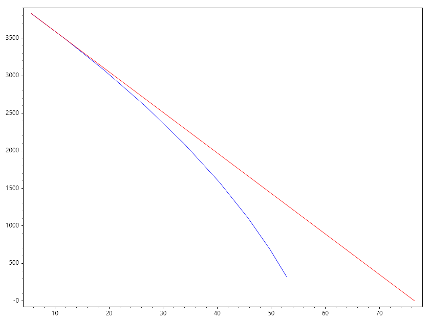
ColVec Z = Arrayfun(p => ZfactorHY(p/P_pc, Tr), P);
ColVec PZ = P.Div(Z);
double m = (PZ[^2] - PZ[^1])/(G[^2] - G[^1]);
ColVec Pl = new double[] { PZ[^1], 0 }, Gl = new double[] { G[^1], G[^1] -PZ[^1]/m };
Plot(G, PZ, "b"); HoldOn();
Plot(Gl, Pl, "r"); HoldOff();
SaveAs("Gas_Reservoir_MB.png");
//
Exercise
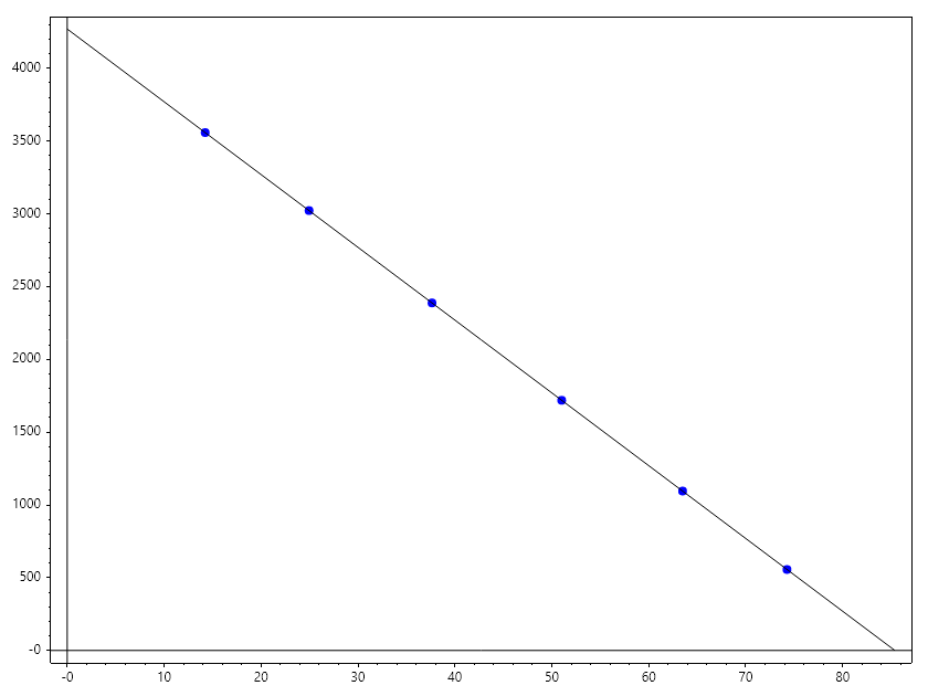
Given the production history of Gas Reservoir below
double[] P = [2500, 2100, 1700, 1300, 900, 500];
double[] G = [14.2314, 24.9498, 37.6355, 51.0163, 63.4889, 74.2625];
double[] Z = [0.7027, 0.6949, 0.7120, 0.7564, 0.8219, 0.8988];

double[] PZ = [.. P.Zip(Z, (p, z) => p/z)];

var p = Polyfit(G, PZ, 1);
double GIIP = -p[1]/p[0];
Console.WriteLine($"Initial P/z = {p[1]}");
Console.WriteLine($"GIIP = {GIIP}");
Scatter(G, PZ, "fob"); HoldOn();
Plot([0, GIIP], [p[1], 0], "k");
Hline(0); Vline(0);
HoldOff();
SaveAs("Gas_Reserve_Exercise.png");
Ouput
Initial P/z = 4269.359990640229
GIIP = 85.38985191375376
Determine the type of the reservoir
Estimate the Initial Gas In-place