Orthogonal Polynomials

Legendre Functions

Legendre polynomials are a set of orthogonal polynomials that arise in solving certain types of differential equations, particularly in physics and engineering. They are named after the French mathematician Adrien-Marie Legendre.

The Legendre polynomials \(P_n(x)\) are solutions to Legendre’s differential equation:

\[(1 - x^2) \frac{d^2y}{dx^2} - 2x\frac{dy}{dx} + n(n+1)y = 0\]

where: math:n is a non-negative integer.

Some key properties of Legendre polynomials include:

Orthogonality: They are orthogonal with respect to the weight function \(w(x) = 1\) on the interval \([-1,1]\).
Normalization: \(P_n(1) = 1\) for all \(n\)
Recurrence Relation: They satisfy the recurrence relation:

\[(n+1)P_{n+1}(x) = (2n + 1)xP_{n}(x) - nP_{n-1}(x)\]

Types of Legendre polynomials

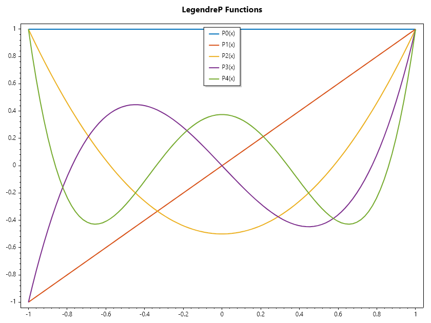
Legendre polynomials of the First Kind \((P_n(x))\)

\[P_n(z) = \frac{1}{2^n}\sum_{k=0}^{\lfloor \frac{n}{2} \rfloor} \frac{(-1)^k(2n-2k)!}{k!(n-k)!(n - 2k)!}x^{n-2k}\]

ColVec x = Linspace(-1, 1);
Indexer Z = new(0, 5);
Matrix P = Z.Select(z => LegendreP(z, x)).ToList();
Plot(x, P, Linewidth: 2);
Title("LegendreP Functions");
Legend(Z.Select(z => $"P{z}(x)"), UpperCenter);
SaveAs("LegendreP-Functions.png");

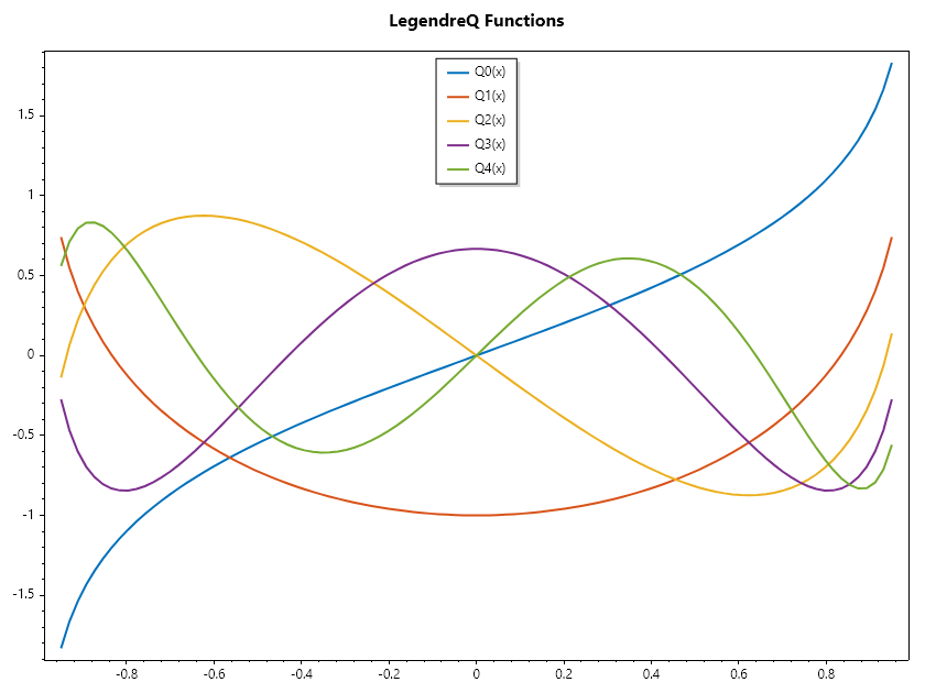
Legendre polynomials of the Second Kind \((Q_n(x))\)

\[Q_n(z) = \frac{1}{2}P_n(x)\ln\left(\frac{1+x}{1-x}\right) + \sum_{k=1}^{\lfloor \frac{n+1}{2} \rfloor} \frac{2n - 4k + 3}{(2k - 1)(n - k + 1)}P_{n - 2k + 1}(x)\]

ColVec x = Linspace(-0.95, 0.95);
Indexer Z = new(0, 5);
Matrix Q = Z.Select(z => LegendreQ(z, x)).ToList();
Plot(x, Q, Linewidth: 2);
Title("LegendreQ Functions");
Legend(Z.Select(z => $"Q{z}(x)"), UpperCenter);
SaveAs("LegendreQ-Functions.png");

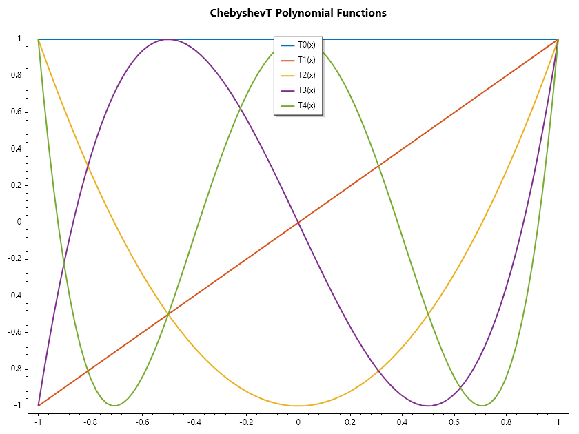
Chebyshev polynomials

Chebyshev polynomials are a sequence of orthogonal polynomials that are widely used in numerical analysis, approximation theory, and other areas of mathematics. There are two main types of Chebyshev polynomials: those of the first kind, denoted as \(T_n(x)\) and those of the second kind, denoted as \(U_n(x)\).

Types of Chebyshev polynomials

ChebyshevT polynomials of the First Kind \((T_n(x))\)

\[\begin{split}\begin{array}{rcl} T_0(x) &=& 1 \\ T_1(x) &=& x \\ T_{n+1}(x) &=& 2xT_n(x) - T_{n-1}(x) ~\text{for}~ n \geq 1 \end{array}\end{split}\]

ColVec x = Linspace(-1, 1);
Indexer Z = new(0, 5);
Matrix T = Z.Select(z => ChebyshevT(z, x)).ToList();
Plot(x, T, Linewidth: 2);
Title("ChebyshevT Polynomial Functions");
Legend(Z.Select(z => $"T{z}(x)"), UpperCenter);
SaveAs("ChebyshevT-Polynomial-Functions.png");

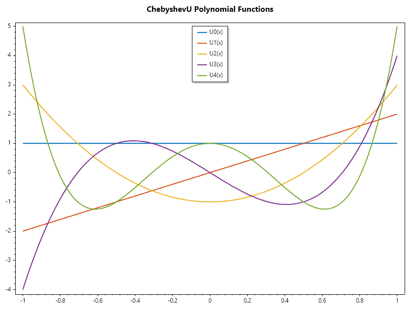
ChebyshevU polynomials of the Second Kind \((U_n(x))\)

\[\begin{split}\begin{array}{rcl} U_0(x) &=& 1 \\ U_1(x) &=&2x \\ U_{ n+1} (x) &=&2xU_n(x) - U_{ n-1} (x) ~\text{ for} ~n \geq 1 \end{array}\end{split}\]

ColVec x = Linspace(-1, 1);
Indexer Z = new(0, 5);
Matrix T = Z.Select(z => ChebyshevU(z, x)).ToList();
Plot(x, T, Linewidth: 2);
Title("ChebyshevU Polynomial Functions");
Legend(Z.Select(z => $"U{z}(x)"), UpperCenter);
SaveAs("ChebyshevU-Polynomial-Functions.png");

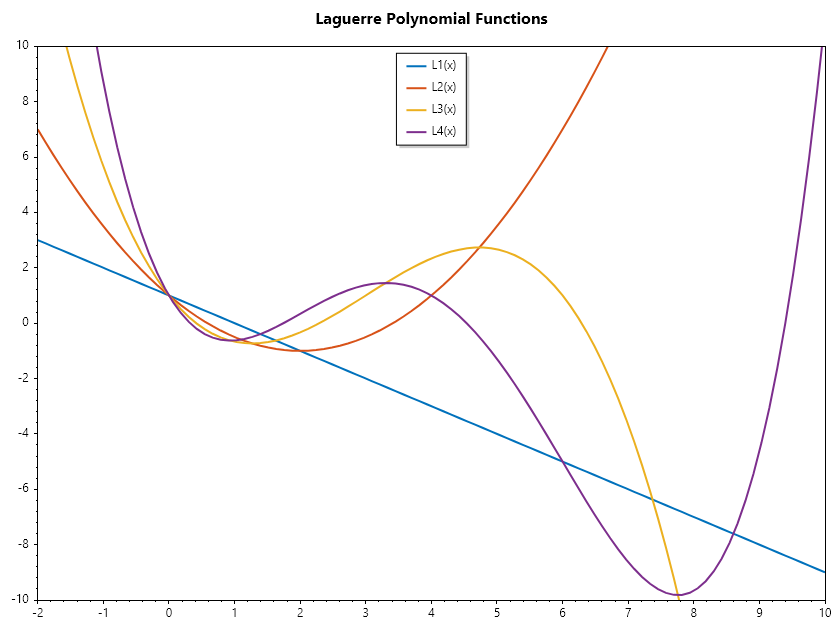
Laguerre Polynomial

Laguerre polynomials are a sequence of orthogonal polynomials named after the French mathematician Edmond Laguerre. These polynomials are solutions to the Laguerre differential equation:

\[x \cfrac{d^2y}{dx^2} + (1 - x)\cfrac{dy}{dx} + ny = 0\]

where: math:n is a non-negative integer. The Laguerre polynomials are denoted by \(L_n(x)\) and have several important properties and applications.

It can be generated by the following recurrent relation

\[\begin{split}\begin{array}{rcl} L_0(x) &=& 1 \\ L_1(x) &=& 1 - x \\ (n + 1)L_{n+1}(x) &=& (2n + 1 - x)L_n(x) - nL_{n-1}(x) ~\text{for}~ n \geq 1 \end{array}\end{split}\]

ColVec x = Linspace(-2, 10);
Indexer Z = new(1, 5);
Matrix P = Z.Select(z => Laguerre(z, x)).ToList();
Plot(x, P, Linewidth: 2);
Title("Laguerre Polynomial Functions");
Axis([-2, 10, -10, 10]);
Legend(Z.Select(z => $"L{z}(x)"), UpperCenter);
SaveAs("Laguerre-Polynomial-Functions.png");

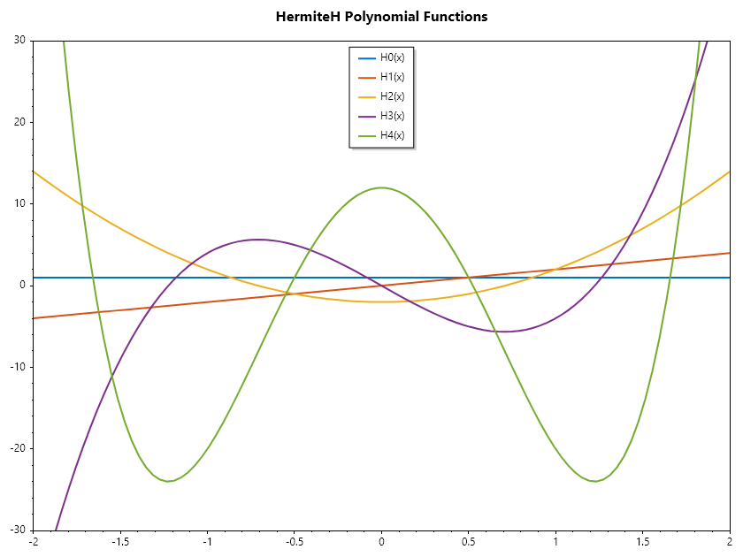
Hermite Polynomials

Hermite polynomials are a classical sequence of orthogonal polynomials that arise in various fields of mathematics and physics. Named after the French mathematician Charles Hermite, these polynomials are particularly significant in probability theory, combinatorics, and quantum mechanics.

\[x \cfrac{d^2y}{dx^2} - 2x\cfrac{dy}{dx} + 2ny = 0\]

where \(n\) is a non-negative integer. The Hermite polynomials are denoted by \(H_n(x)\) and have several important properties and applications. It can be generated by the following recurrent relation

\[\begin{split}\begin{array}{rcl} H_0(x) &=& 1 \\ H_1(x) &=& 2x \\ H_{n+1}(x) &=& 2x H_n(x) - 2n H_{n-1}(x) ~\text{for}~ n \geq 1 \end{array}\end{split}\]

ColVec x = Linspace(-2, 2);
Indexer Z = new(0, 5);
Matrix T = Z.Select(z => HermiteH(z, x)).ToList();
Plot(x, T, Linewidth: 2);
Title("HermiteH Polynomial Functions");
Axis([-2, 2, -30, 30]);
Legend(Z.Select(z => $"H{z}(x)"), UpperCenter);
SaveAs("HermiteH-Polynomial-Functions.png");