Error Functions
Error Function (\(\text{erf}\))
The error function \(\text{erf}(x)\) is a non-elementary function that occurs in probability, statistics, and partial differential equations. It represents the integral of the Gaussian (Normal) distribution.
Definition: \(\text{erf}(x) = \cfrac{2}{\sqrt{\pi}} \int_0^x e^{-t^2} dt\)
Asymptotes: The function approaches \(1\) as \(x \to \infty\) and
\(-1\) as \(x \to -\infty\). * Physics: It is the primary solution for heat diffusion problems in infinite or semi-infinite media where an initial temperature step exists.
ColVec x = Linspace(-3, 3, 200);
Plot(x, Erf(x), "b", 2);
//Hline(1); Hline(-1);
Title("Error Function erf(x)");
Xlabel("x"); Ylabel("erf(x)");
SaveAs("Error.png");

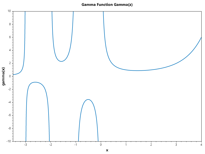
Gamma Function \(\Gamma(z)\)
The Gamma function generalizes the factorial to real and complex numbers. For any positive integer \(n\), \(\Gamma(n) = (n-1)!\).
Functional Equation: \(\Gamma(z+1) = z\Gamma(z)\).
LnGamma: Because \(\Gamma(z)\) grows extremely fast, the natural logarithm of Gamma (\(\text{Log-Gamma}\)) is used in computation to prevent floating-point overflow.
ColVec x = Linspace(-3.5, 4, 1000);
//Masking values near poles for a cleaner plot
ColVec y = Gamma(x);
y[Abs(y) > 20] = double.NaN;
Plot(x, y, "p", 2);
Axis([-3.5, 4, -10, 10]);
Title("Gamma Function Gamma(z)");
Xlabel("x"); Ylabel("gamma(x)");
SaveAs("Gamma.png");
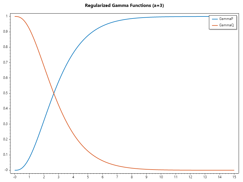
Regularized Incomplete Gamma (P and Q)
These are the normalized versions of the incomplete Gamma integral, ensuring the output stays within the range \([0, 1]\).
Lower Regularized (P):
Upper Regularized (Q):
Relationship:
These are the CDF and Survival functions of the Gamma distribution.
ColVec x = Linspace(0, 15, 200);
double a = 3.0;// Shape parameter
Plot(x, Hcart(GammaP(a, x), GammaQ(a, x)), Linewidth: 2);
Title($"Regularized Gamma Functions (a={a})");
Legend(["GammaP", "GammaQ"]);
SaveAs("IncGamma.png");
LnGamma \(\text{LnGamma}\)
Definition and Purpose
The :math:text{LnGamma} function, denoted as \(\ln\Gamma(z)\), is the natural logarithm of the Gamma function. While it might seem redundant to have a separate function for the log of an existing function, it is essential for numerical computing.
The Overflow Problem: The Gamma function \(\Gamma(z)\) grows at a “factorial” rate. For example, \(\Gamma(172)\) is approximately \(1.24 \times 10^{307}\), which is the limit of double-precision floating-point numbers. Any value larger than 171 will result in an Inf (overflow) error.
The Solution: By working in “log-space,” we can handle calculations involving massive factorials without crashing the program.
Mathematical Properties
Stirling’s Approximation: For large \(z\), \(\text{LnGamma}\) is often approximated as:
Derivatives: The first derivative of \(\ln\Gamma(z)\) is called the Digamma function (\(\psi\)), and the second derivative is the Trigamma function. The general derivative of order n is the Polygamma function.
Application: Bayesian Statistics
In Bayesian inference and likelihood calculations, we often multiply many probabilities together, many of which involve Gamma functions (like in the Beta or Gamma distributions). Multiplying many tiny numbers leads to “underflow.” Instead, we sum the \(\text{LnGamma}\) values to stay within a safe numerical range.
// Demonstrate the benefit of gammaln over log(gamma)

ColVec x = 1..200;

// This will fail/overflow after x = 171
ColVec y_gamma = Gamma(x),   y_log_gamma = Log(y_gamma);

// This will work perfectly for all values
ColVec y_gammaln = LnGamma(x);

Plot(x, Hcart(y_gammaln, y_log_gamma), Linewidth: 2);
Title("LnGamma Function");
Xlabel("x"); Ylabel("Ln(Gamma(x))");
Legend(["gammaln(x)", "log(gamma(x)) - Note the break at x=171"]);
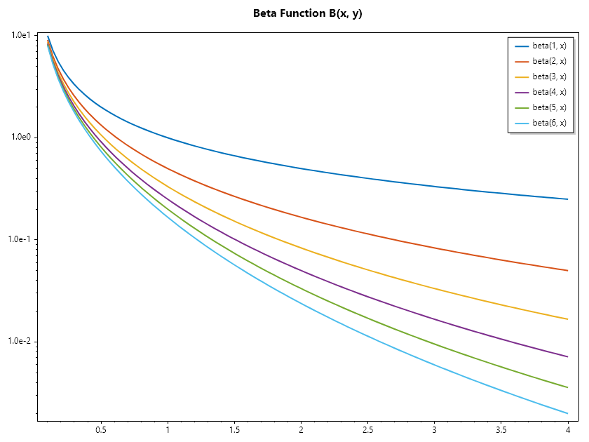
Beta Function \(B(x, y)\)
The Beta function, also known as the Euler integral of the first kind, is closely related to the Gamma function and binomial coefficients.
Identity: \(B(x, y) = \cfrac{\Gamma(x)\Gamma(y)}{\Gamma(x+y)}\)
Application: Used extensively in Bayesian inference as the conjugate prior for Bernoulli and Binomial distributions.
Indexer b = 1..7;
ColVec x = Linspace(0.1, 4, 100);
Matrix y = b.Select(b => Beta(b, x)).ToList();
SemiLogy(x, y, Linewidth: 2);
Title("Beta Function B(x, y)");
Legend(b.Select(b => $"beta({b}, x)"));
SaveAs("Beta.png");
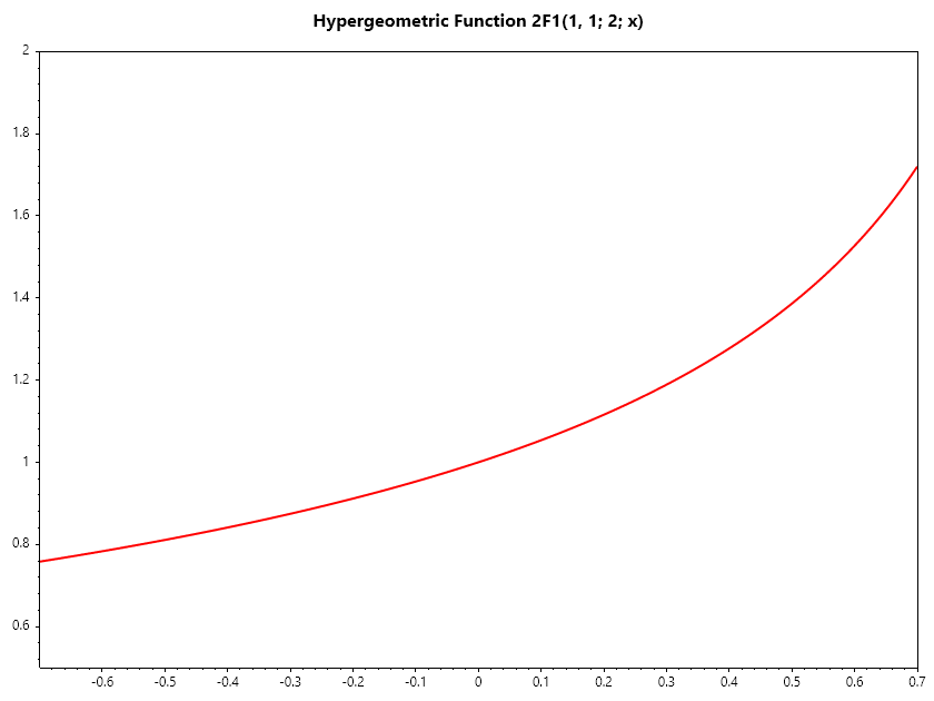
Generalized Hypergeometric Function \({}_pF_q\)
This series provides a unified framework for almost all special functions. By varying the number and values of numerator (\(p\)) and denominator (\(q\)) parameters, one can derive Bessel, Legendre, and Laguerre functions.
Pochhammer Symbol: The series uses rising factorials \((a)_n\).
Gauss Hypergeometric: The most common form is \({}_2F_1(a, b; c; z)\).
ColVec x = Linspace(-0.7, 0.7, 200);
ColVec y = HyperGeom([1, 1], [2], x); // This specific case equals -log(1-x)/x
Plot(x, y, "r", Linewidth: 2);
Axis([-0.7, 0.7, 0.5, 2]);
Title("Hypergeometric Function 2F1(1, 1; 2; x)");
SaveAs("Hypergeomtric.png");