Higher Order Differential Equations
Introduction
A higher‑order differential equation involves derivatives of order two or higher. Many physical systems such as oscillations, mechanical vibrations, and electrical circuits are naturally modeled by second‑order or higher‑order equations.
Examples:
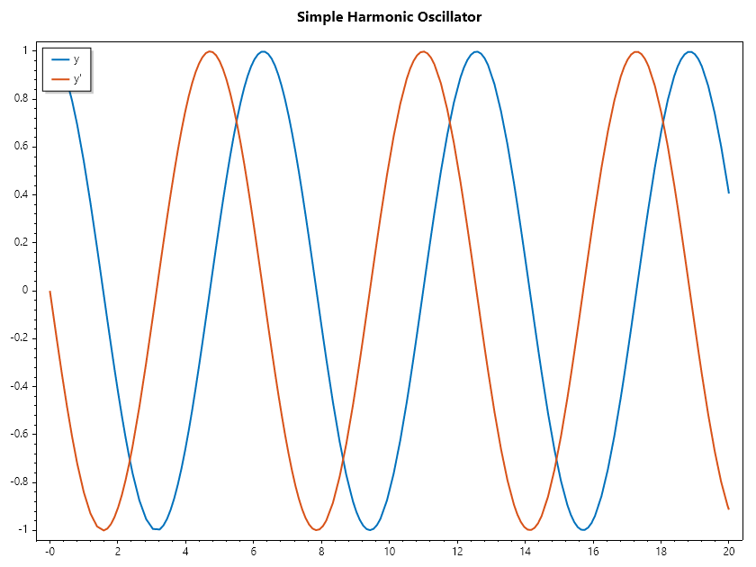
Simple harmonic oscillator (second order)
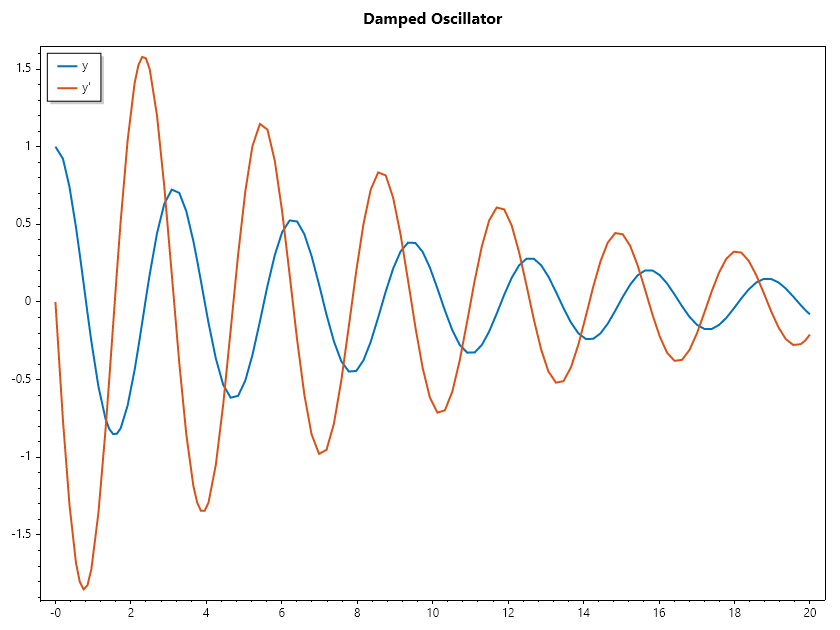
Damped oscillator
Forced oscillator
Beam deflection problems
RLC electrical circuits
To use SepalSolver to solve higher‑order ODEs, they have to first be converted into equivalent systems of first‑order equations.
General Form
A general n‑th order ODE can be written as:
To solve with SepalSolver, we introduce variables:
Then the system becomes:
// Define the ODE system as a function
double[] dydt(double t, double[] y) => [y[1], y[2], ..., f(t,y)];
Examples
Here are examples of converting and solving various higher‑order ODEs using SepalSolver.
Example 1 : Simple Harmonic Oscillator (Second Order)
double[] dydt(double t, double[] y) => [ y[1], -y[0] ];
double[] y0 = [1.0, 0.0]; // y(0)=1, y'(0)=0
double[] tspan = [0, 20];
(ColVec T, Matrix Y) = Ode45(dydt, y0, tspan);
Plot(T, Y, Linewidth: 2);
Legend(["y", "y'"], UpperLeft);
Title("Simple Harmonic Oscillator");
SaveAs("HigherOrder_SHO.png");
Example 2 : Damped Oscillator
double beta = 0.1, omega = 2.0;
double[] dydt(double t, double[] y) => [ y[1], -2*beta*y[1] - omega*omega*y[0] ];
double[] y0 = [1.0, 0.0];
double[] tspan = [0, 20];
(ColVec T, Matrix Y) = Ode45(dydt, y0, tspan);
Plot(T, Y, Linewidth: 2);
Legend(["y", "y'"], UpperLeft);
Title("Damped Oscillator");
SaveAs("HigherOrder_Damped.png");
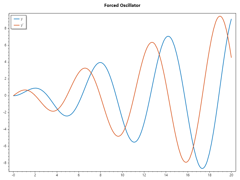
Example 3 : Forced Oscillator
double[] dydt(double t, double[] y) => [ y[1], -y[0] + Cos(t) ];
double[] y0 = [0.0, 0.0];
double[] tspan = [0, 20];
(ColVec T, Matrix Y) = Ode45(dydt, y0, tspan);
Plot(T, Y, Linewidth: 2);
Legend(["y", "y'"], UpperLeft);
Title("Forced Oscillator");
SaveAs("HigherOrder_Forced.png");
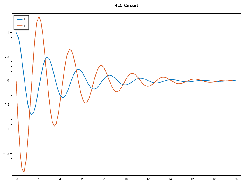
Example 4 : RLC Circuit
 double L = 1.0, R = 0.5, C = 0.2;
 double[] dydt(double t, double[] i) => [ i[1], -(R/L)*i[1] - (1.0/(L*C))*i[0] ];
 double[] i0 = [1.0, 0.0];
 double[] tspan = [0, 20];
 (ColVec T, Matrix Y) = Ode45(dydt, i0, tspan);
 Plot(T, Y, Linewidth: 2);
 Legend(["i", "i'"], UpperLeft);
Title("RLC Circuit");
 SaveAs("HigherOrder_RLC.png");
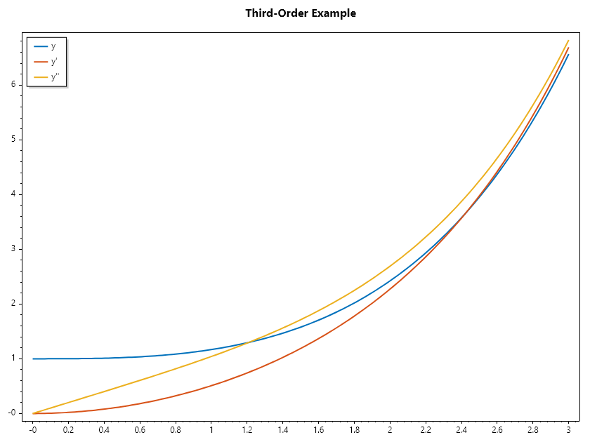
Example 5 : Third‑Order Example
double[] dydt(double t, double[] y) => [ y[1], y[2], y[0] ];
double[] y0 = [1.0, 0.0, 0.0];
double[] tspan = [0, 3];
(ColVec T, Matrix Y) = Ode45(dydt, y0, tspan);
Plot(T, Y, Linewidth: 2);
Legend(["y", "y'", "y''"], UpperLeft);
Title("Third‑Order Example");
SaveAs("HigherOrder_Third.png");
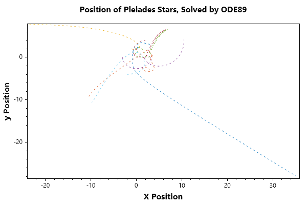
Example 6 : Pleiades System (Using Higher Order Solvers)
The Pleiades, also known as the Seven Sisters(M45)[1], is a prominent open star cluster located in the constellation Taurus.It’s one of the closest and most easily visible star clusters to Earth[2], making it a favorite target for stargazers and a subject of fascination across cultures. The system of equations describing the motion of the stars in the cluster consists of 14 nonstiff second-order differential equations, which produce a system of 28 equations when rewritten in first-order form.
Celestial mechanics is basically an interplay between
Newton’s law of gravitation: \(F_i = \sum_{i \neq j} g \cfrac{m_i m_j}{||p_j - p_i||^2}d_{ij}\) and
Newton’s second law of motion: \(F_i = m_i\cfrac{ d^2p_i}{ dt^2}\).
The positions determine the gravitational forces acting on the bodies, but the net force on each of the bodies determines its acceleration(i.e.changes its position from the second order).
we examine this system in 2D, i.e. \(p_i = [x_i, y_i]\), \(d_{ij} = \cfrac{(p_j - p_i)}{r_{ ij}}\) and \(r_{ij} = ||p_j - p_i||\)
The dynamics of the system can then be modelled as:
// define masses
double[] m = [1, 2, 3, 4, 5, 6, 7];

// define function
double[] pleiades(double t, double[] q)
{
    double[] dqdt = new double[28];
    double x1, x2, y1, y2, dx, dy, r3;
    for (int i = 0; i < 7; i++)
    {
        // x- velocity of star i
        dqdt[i + 0] = q[i + 14];
        // y- velocity of star j
        dqdt[i + 7] = q[i + 21];
        x1 = q[i]; y1 = q[i + 7];
        for (int j = 0; j < 7; j++)
        {
            x2 = q[j]; y2 = q[j + 7];
            if (j != i)// The star does not attract itself
            {
                dx = x2 - x1; dy = y2 - y1;
                r3 = Pow(dx * dx + dy * dy, 1.5);
                //impact of star j on x-acceleration of star i
                dqdt[i + 14] += m[j] * dx / r3;
                //impact of star j on y-acceleration of star i
                dqdt[i + 21] += m[j] * dy / r3;
            }
        }
    }
    return dqdt;
}

double[] init = [3, 3,-1, -3, 2, -2, 2,
                 3, -3, 2, 0, 0, -4, 4,
                 0, 0, 0, 0, 0, 1.75, -1.5,
                 0, 0, 0, -1.25, 1, 0, 0];

double[] tspan = Linspace(1, 15, 200);
var opts = Odeset(AbsTol: 1e-15, RelTol: 1e-13);
Figure(600, 400);
(ColVec T, Matrix Y) = Ode89(pleiades, init, tspan, opts);
Plot(Y[.., 0..7], Y[.., 7..14], ":");
Title("Position of Pleiades Stars, Solved by ODE89");
Xlabel("X Position"); Ylabel("y Position");
SaveAs("Position-of-Pleiades-Stars-Ode89.png");

HoldOn();
ScatterHandle[] Stars = [..Enumerable.Range(0,7).Select(j =>
                            Scatter(Y[0, j], Y[0, j + 7], "fo", 20))];
HoldOff();


byte[] Animfun(int i)
{
    for (int j = 0; j < 7; j++)
    {
        Stars[j].Xdata = Y[i, j];
        Stars[j].Ydata = Y[i, j + 7];
    }
    return GetFrame();
}
AnimationMaker(Animfun, "Position-of-Pleiades-Stars-CCL-Math-Ode89.gif", 10, 200);
CloseFig();