First Order Differential Equation
1. What is a Differential Equation?
A differential equation(DE) is a mathematical equation that relates a function with its derivatives. In simpler terms, it describes how a quantity changes in relation to its current state.
The Function: \((y)\): Represents the “state” of a system(e.g., the position of a car, the temperature of a room).
The Derivative: \(\cfrac{dt}{dy}\) Represents the “rate of change”(e.g., the speed of the car, how fast the room is cooling).
An ODE is “Ordinary” because the unknown function depends on only one independent variable(usually time t or distance x).
2. The Intuition: The Slope Field
If you have an equation like \(\cfrac{dt}{dy} = y\), the equation is telling you: “The steeper the graph gets, the higher the value of y must be.” Even before solving an equation, we can visualize it using a Slope Field(or Direction Field).At every point(t, y) on a graph, we draw a tiny line segment with the slope dictated by the differential equation. A solution to the ODE is simply a curve that “follows the arrows.”
3. Analytical vs.Numerical Solutions
Analytical Solutions(The “Exact” Way) This is what you do in a calculus class. You use integration techniques to find a precise formula for y(t).
example: For \(\cfrac{dt}{dy} = ky\), the analytical solution is \(y(t) = Ce^{kt}\)
Pros: Perfectly accurate; gives you a formula you can use forever.
Cons: Most complex equations in physics and engineering cannot be solved this way.
Numerical Solutions (The “Approximate” Way) When an equation is too “messy” for calculus, we use numerical methods.Instead of finding a pretty formula, we use a computer to start at an initial point and take tiny steps forward, calculating the slope as we go.
Pros: Can solve almost any equation, no matter how complex.
Cons: Always contains a small amount of “truncation error” because we are approximating a smooth curve with small straight lines.
4. The Anatomy of an Initial Value Problem (IVP)
To get a single, specific answer from an ODE, you need a starting point, known as the Initial Condition. The Equation: \(\cfrac{dt}{dy} = f(t, y)\) (The rule of change), The Initial Condition: \(y(0)=y_0\) (The starting point). Without a starting point, a differential equation has an infinite number of solutions(a “family” of curves). The initial condition picks the specific path the system takes. Numerical methods are essential because most real-world ordinary differential equations (ODEs) cannot be solved analytically (with pen and paper). Instead of finding a continuous formula for \(y(x)\), we calculate discrete values at specific points. This guide covers the use of sepalsolver for solving an Initial Value Problem (IVP) defined by: \(\cfrac{dy}{dt} = f(t, y), \quad y(t_0) = y_0\) where \(f(t, y)\) is a function that defines the rate of change of \(y\) with respect to \(t\), and \(y_0\) is the initial value of \(y\) at time \(t_0\).
Examples
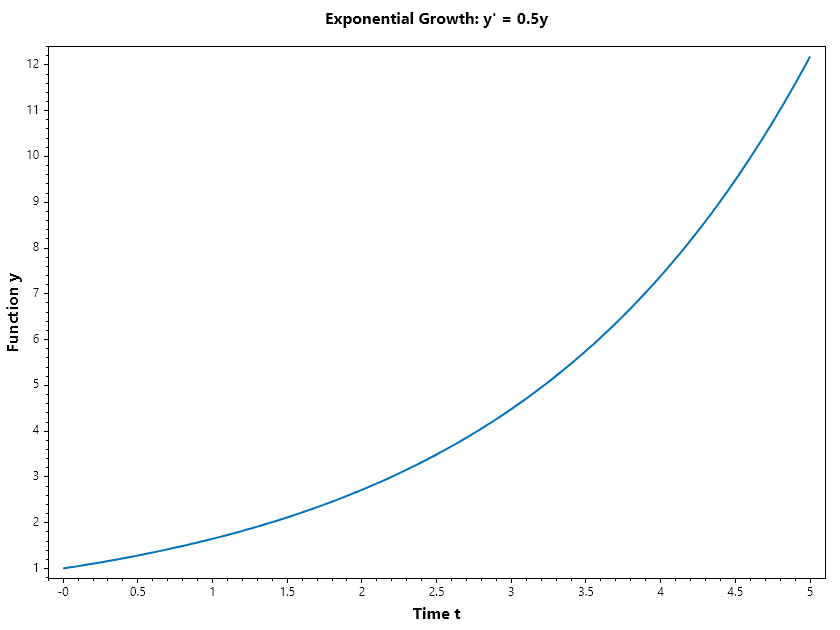
Example 1 : Exponential Growth
// Define the ODE as a function
double dydt(double t, double y) => 0.5*y;
// Initial condition
double y0 = 1;
// Time span
double[] tspan = [0, 5];
// Solve the ODE using Ode45
(ColVec T, ColVec Y) = Ode45(dydt, y0, tspan);
// Plot the results
Plot(T, Y, Linewidth: 2);
Title("Exponential Growth: y' = 0.5y");
Xlabel("Time t");
Ylabel("Function y");
SaveAs("Exponential_Growth.png");
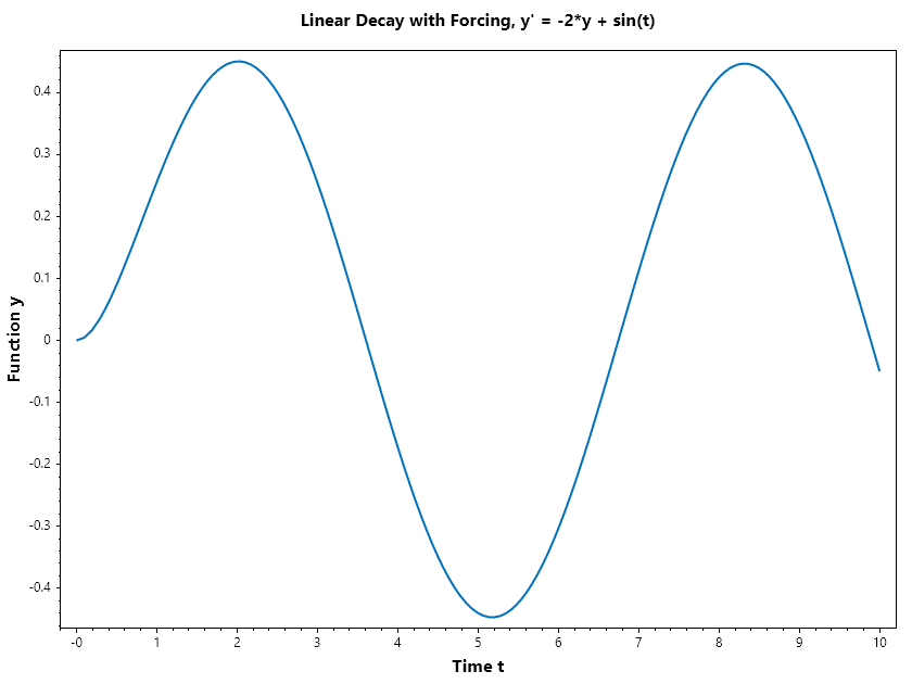
Example 2 : Linear Decay with Forcing
// Define the ODE as a function
double dydt(double t, double y) => -2*y + Sin(t);
// Initial condition
double y0 = 0;
// Time span
double[] tspan = [0, 10];
// Solve the ODE using Ode45
(ColVec T, ColVec Y) = Ode45(dydt, y0, tspan);
// Plot the results
Plot(T, Y, Linewidth: 2);
Title("Linear Decay with Forcing, y' = -2*y + sin(t)");
Xlabel("Time t");
Ylabel("Function y");
SaveAs("Linear_Decay_with_Forcing.png");
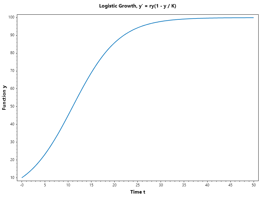
Example 3 : Logistic Growth
// Define the ODE as a function
double r = 0.2, K = 100;
double dydt(double t, double y) => r * y * (1 - y / K);
// Initial condition
double y0 = 10;
// Time span
double[] tspan = [0, 50];
// Solve the ODE using Ode45
(ColVec T, ColVec Y) = Ode45(dydt, y0, tspan);
// Plot the results
Plot(T, Y, Linewidth: 2);
Title("Logistic Growth, y' = ry(1 - y / K)");
Xlabel("Time t");
Ylabel("Function y");
SaveAs("Logistic_Growth.png");
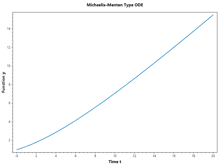
Example 4 : Michaelis–Menten Type ODE
// Define the ODE as a function
double Vmax = 1.0, K = 2.0;
double dydt(double t, double y) => (Vmax * y) / (K + y);
// Initial condition
double y0 = 1;
// Time span
double[] tspan = [0, 20];
// Solve the ODE using Ode45
(ColVec T, ColVec Y) = Ode45(dydt, y0, tspan);
// Plot the results
Plot(T, Y, Linewidth: 2);
Title("Michaelis–Menten Type ODE");
Xlabel("Time t");
Ylabel("Function y");
SaveAs("Michaelis_Menten_Type_ODE.png");
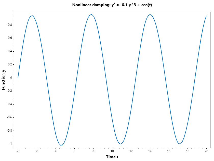
Example 5 : NonLinear Damping
// Define the ODE as a function
double dydt(double t, double y) => -0.1 * Pow(y, 3) + Cos(t);
// Initial condition
double y0 = 0;
// Time span
double[] tspan = [0, 20];
// Solve the ODE using Ode45
(ColVec T, ColVec Y) = Ode45(dydt, y0, tspan);
// Plot the results
Plot(T, Y, Linewidth: 2);
Title("Nonlinear damping: y' = -0.1 y^3 + cos(t)");
Xlabel("Time t");
Ylabel("Function y");
SaveAs("Non_Linear_Damping.png");