Hemite Spline

Hermite Interpolation

Hermite Interpolation is a method of interpolating data points that accounts for not only the values of the function but also the values of its derivatives. While standard linear or polynomial interpolation only ensures the curve passes through the points \((x_i, y_i)\). Hermite interpolation ensures the curve matches the “slope”(tangent) at those points as well. This results in a much smoother and more physically realistic transition between points, particularly in motion planning or structural deflection models where velocity or tangency must be continuous.

1. The Cubic Hermite Spline

The most common form is the Cubic Hermite Spline. For a single interval between \(x_0\) and \(x_1\) the interpolant is a third-degree polynomial.To construct it, we need four pieces of information: * The starting and ending values: \(y_0\) and \(y_1\) * The starting and ending derivatives (slopes): \(y'_0\) and \(y'_1\)

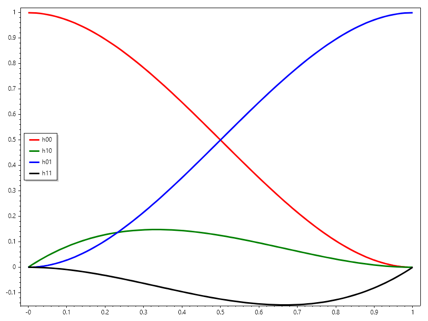
The resulting curve is expressed using Hermite Basis Functions, which act as weights for the coordinates and the slopes.

ColVec t = Linspace(0, 1), t2 = t.Pow(2), t3 = t.Pow(3);
ColVec h00 = 2 * t3 - 3 * t2 + 1, h10 = t3 - 2 * t2 + t,
       h01 = -2 * t3 + 3 * t2, h11 = t3 - t2;

Plot(t, h00, "r", 3); HoldOn();
Plot(t, h10, "g", 3);
Plot(t, h01, "b", 3);
Plot(t, h11, "k", 3); HoldOff();
Legend(["h00", "h10", "h01", "h11"], MiddleLeft);
SaveAs("hermite_modes.png");

2. Implementation in SepalSolver

In SepalSolver, Hermite interpolation is often used when the user provides a “slope vector” alongside their dataset. This is common in trajectory generation where you know where a robot should be and how fast it should be moving at that specific moment.

double[] x = [0.0, 1.0];
double[] y = [0.0, 10.0];
double[] dy = [0.0, 0.0]; // Zero velocity at start and end

// Estimate value at x = 0.5
double xq = 0.5;

// Manually implementing Hermite interpolation
double x0 = x[0], x1 = x[1], y0 = y[0], y1 = y[1], m0 = dy[0], m1 = dy[1];
double dx = x1 - x0, t = (xq - x0) / dx, t2 = t * t, t3 = t2 * t;
double h00 = 2 * t3 - 3 * t2 + 1,
       h10 = t3 - 2 * t2 + t,
       h01 = -2 * t3 + 3 * t2,
       h11 = t3 - t2;
double result = h00 * y0 + h10 * dx * m0 + h01 * y1 + h11 * dx * m1;

// Because slopes are 0, this creates an S-curve rather than a straight line
Console.WriteLine($"Smooth transition value: {result}");

Ouput

Smooth transition value: 5

Examples

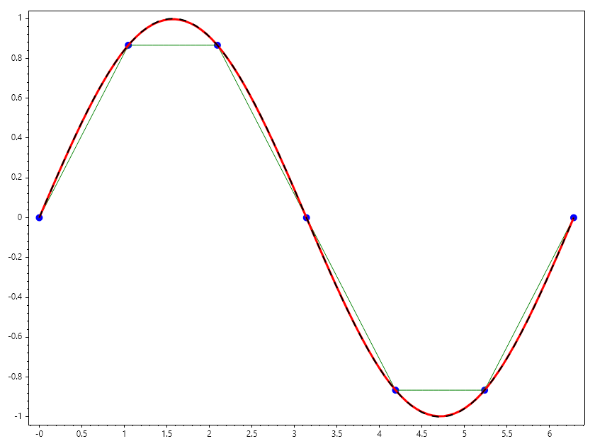
Example 1 : Compare Linear and Hermite interpolation for sparsely compited sin(x)

If sin(x) is give at 7 points between \(0\) and \(\pi\). Interpolate for sin(x) for 100 points between \(0\) and \(\pi\) using linear and hermite spline and compare the plots.

// Using linear interpolation
ColVec x = Linspace(0, 2*pi, 7), s = Sin(x);
ColVec xq = Linspace(0, 2*pi), sq = Interp1(x, s, xq);
Scatter(x, s, "fob", 10); HoldOn();
Plot(xq, sq, "g");

// using hermite interpolation
int j = 1;
ColVec c = Cos(x);

ColVec sh = Zeros(xq.Numel);
for (int i = 0; i < xq.Numel; i++)
{
    while (xq[i] > x[j]) j++;

    double x0 = x[j-1], x1 = x[j], y0 = s[j-1], y1 = s[j], m0 = c[j-1], m1 = c[j];
    double dx = x1 - x0, t = (xq[i] - x0) / dx, t2 = t * t, t3 = t2 * t;

    double h00 = 2 * t3 - 3 * t2 + 1,
           h10 = t3 - 2 * t2 + t,
           h01 = -2 * t3 + 3 * t2,
           h11 = t3 - t2;
    sh[i] = h00 * y0 + h10 * dx * m0 + h01 * y1 + h11 * dx * m1;
}
Plot(xq, sh, "r", 3);
Plot(xq, Sin(xq), "--k", 2); HoldOff();
SaveAs("hermite_vs_linear.png");

Example 2 :

If a robot moves from point A to point B, a linear path causes an abrupt change in velocity at the corners. By using Hermite interpolation and specifying the desired entry/exit velocity vectors, we create a path that the robot can follow without stopping or jerking.

double[] t = [0, 5, 10];    // Time
double[] pos = [0, 20, 50]; // Position
double[] vel = [0, 10, 0];  // Specific velocities at those times

Key Difference: Hermite vs. Cubic Spline

Exercise: Animation of Slope Impact

Task: Observe how changing the slope \(dy\) at the first point affects the plot of the function.

//define hemitespline function
double[] HermiteFun(double[] x, double[] y, double[] dy, double[] xq)
{
    double[] yq = new double[xq.Length];
    int j = 1;
    for (int i = 0; i < xq.Length; i++)
    {
        while (xq[i] > x[j]) j++;

        double x0 = x[j-1], x1 = x[j], y0 = y[j-1], y1 = y[j], m0 = dy[j-1], m1 = dy[j];
        double dx = x1 - x0, t = (xq[i] - x0) / dx, t2 = t * t, t3 = t2 * t;

        double h00 = 2 * t3 - 3 * t2 + 1,
               h10 = t3 - 2 * t2 + t,
               h01 = -2 * t3 + 3 * t2,
               h11 = t3 - t2;
        yq[i] = h00 * y0 + h10 * dx * m0 + h01 * y1 + h11 * dx * m1;
    }
    return yq;
}

// define x and y
double[] x = [0, 1];
double[] y = [0, 0];

// start with this slope
double[] dy = [-1, 1];

// define querry points
double[] xq = Linspace(0, 1);
double[] yq = HermiteFun(x, y, dy, xq);

// plot the result.
var plt = Plot(xq, yq, Linewidth: 2);
Axis([0, 1, -0.3, 0.2]);

// set up animation function
byte[] animfun(int i)
{
    dy[0] = Sin(pi + i * 0.02*pi);           // increase the starting slope
    plt.Ydata = HermiteFun(x, y, dy, xq);    // update interpolated values
    return GetFrame();                       //  return the frame
}

// Animate the plot
AnimationMaker(animfun, "Impact_of_changing_slope_at_x_0.gif", 30, 100);

</example 4>

Example 5 : Using Hermite Spline as Sin Approximator

Lets use table of Sine and Cosine at 15 degrees interval given in table

Angle (°)	Sine (\(\sin\))	Cosine (\(\cos\))
0°	\(0\)	\(1\)
15°	\(\cfrac{\sqrt{6} - \sqrt{2}}{4}\)	\(\cfrac{\sqrt{6} + \sqrt{2}}{4}\)
30°	\(\cfrac{1}{2}\)	\(\cfrac{\sqrt{3}}{2}\)
45°	\(\cfrac{\sqrt{2}}{2}\)	\(\cfrac{\sqrt{2}}{2}\)
60°	\(\cfrac{\sqrt{3}}{2}\)	\(\cfrac{1}{2}\)
75°	\(\cfrac{\sqrt{6} + \sqrt{2}}{4}\)	\(\cfrac{\sqrt{6} - \sqrt{2}}{4}\)
90°	\(1\)	\(0\)

// compute square roots of 2 and 3;
double sqrt2 = Sqrt(2), sqrt3 = Sqrt(3);

// define arrays of angle, sine and cosines
double[] Sines = [0, sqrt2*(sqrt3-1)/4, 0.5, sqrt2/2, sqrt3/2, sqrt2*(sqrt3+1)/4, 1];
double[] Cosines = [1, sqrt2*(sqrt3+1)/4, sqrt3/2, sqrt2/2, 0.5, sqrt2*(sqrt3-1)/4, 0];

double SineByHermite(double a)
{
    double da = 15;
    int i = (int)(a/da);
    double t = (a - i*da)/da;
    if (t == 0)
        return Sines[i];
    else
    {

        double t2 = t * t, t3 = t2 * t, dx = da*pi/180;
        double y0 = Sines[i], y1 = Sines[i+1], m0 = Cosines[i], m1 = Cosines[i+1];
        double h00 = 2 * t3 - 3 * t2 + 1,  h10 = t3 - 2 * t2 + t,
               h01 = -2 * t3 + 3 * t2,  h11 = t3 - t2;
        return h00 * y0 + h10 * dx * m0 + h01 * y1 + h11 * dx * m1;
    }
}

double[] x = [.. Rand(20).Select(a => 80*a+10)];
Console.WriteLine("""
      Angle  |  Sineapprox  |    Sine
    ---------+--------------+-------------
    """);
foreach (double a in x)
    Console.WriteLine($"""
          {a:F2}  |   {SineByHermite(a):F6}   |  {Sin(a*pi/180):F6}
        """);

Ouput

  Angle  |  Sineapprox  |    Sine
---------+--------------+-------------
61  |   0.494085   |  0.494086
95  |   0.798060   |  0.798069
15  |   0.767753   |  0.767761
75  |   0.337904   |  0.337907
72  |   0.370137   |  0.370141
88  |   0.729936   |  0.729937
76  |   0.999991   |  0.999991
16  |   0.998770   |  0.998775
88  |   0.372698   |  0.372703
51  |   0.895014   |  0.895020
79  |   0.322147   |  0.322150
01  |   0.974407   |  0.974409
66  |   0.702868   |  0.702868
00  |   0.669078   |  0.669082
46  |   0.736826   |  0.736829
48  |   0.594497   |  0.594504
10  |   0.360061   |  0.360065
11  |   0.516654   |  0.516654
31  |   0.935466   |  0.935476
03  |   0.656412   |  0.656417